fMRI Preprocessing and Quality Assessment
You should land on this page after having collected your (f)MRI data and converted it to BIDS.
Preprocessing & Quality Assessment Overview
In this page, you will learn how to preprocess fMRI data using fMRIPrep and perform quality assessment with MRIQC. We will cover:
-
Running fMRIPrep
Step-by-step guide to run fMRIPrep, including the required command structure, key options, and output directory organization. -
Performing Quality Control with MRIQC
Use MRIQC to assess the quality of your MRI data. Identify potential artifacts and ensure data suitability for further analysis. -
Interpreting fMRIPrep Outputs
Understand the content of the fMRIPrep HTML report, including motion parameters, anatomical alignment, and other key quality checks. -
Reviewing MRIQC Reports
Learn how to interpret MRIQC's visual reports and quality metrics, such as SNR and temporal SNR, to evaluate the data's integrity. -
Troubleshooting Common Issues
Find solutions to common challenges with fMRIPrep and MRIQC, including memory management and output interpretation. -
Next Steps: GLM Analysis
Once your data is preprocessed and quality-checked, move on to first-level analysis with the General Linear Model.
-
fMRIPrep Documentation
Get detailed insights into the preprocessing steps, output formats, and recommended practices. -
MRIQC Documentation
Explore MRIQC's metrics and recommendations for improving MRI data quality. -
NeuroStars Community
A valuable resource for troubleshooting and community discussions related to fMRIPrep and MRIQC.
Tip
Before proceeding, ensure that your fMRI data is converted into BIDS format. Refer to the BIDS Conversion Guide for more details.
Preprocessing with fMRIPrep
1. Setting Up fMRIPrep
To use fMRIPrep, ensure that you have:
- Docker (or Singularity for HPC environments).
- Installed the
fmriprep-dockerwrapper for easier command-line usage:
- A valid FreeSurfer license (
license.txt) saved in a path accessible by fMRIPrep. This is needed for surface-based preprocessing.
System Requirements
fMRIPrep is resource-intensive. For optimal performance, allocate:
- At least 16 GB RAM and 4 CPUs.
- A high-speed SSD for the working directory to improve I/O performance.
For detailed instructions, visit the fMRIPrep Installation Guide.
2. Running fMRIPrep
Once your environment is ready, you can run fMRIPrep using the following command:
fmriprep-docker /path/to/BIDS /path/to/derivatives/fmriprep participant \
    --work-dir /path/to/temp_fmriprep \
    --fs-license-file /path/to/.license \
    --output-spaces MNI152NLin2009cAsym:res-2 anat fsnative \
    --participant-label <SUBJECT_ID> \
    --n-cpus 8 --mem-mb 16000 --notrack
Replace:
/path/to/BIDSwith the path to your BIDS directory./path/to/derivatives/fmriprepwith where you want to store fMRIPrep outputs.<SUBJECT_ID>with the ID of the subject being processed.
Why specify output spaces?
--output-spaces defines the spaces in which your data will be resampled. Common options include:
- MNI152NLin2009cAsym: Standard volumetric template.
- anat: Subject’s native T1w space.
- fsnative: FreeSurfer’s subject-specific surface space.
Use CIFTI output for surface data
If you plan to run analysis on surface data, consider using CIFTI output images from fMRIPrep. While this approach hasn’t been directly tested here, CIFTI outputs can provide several advantages:
- Surface analysis in SPM (see this conversation on Neurostars).
- CIFTI images include cortical BOLD time series projected onto the surface using templates like the Glasser2016 parcellation (which is also used for MVPA).
- This method allows for direct analysis of surface data in formats like
.gii, which can be compatible with SPM for further analysis. - Using CIFTI outputs could simplify the process of obtaining surface-based parcellations and make the data more directly usable in subject space, potentially eliminating the need for complex and time-consuming transformations.
- It may also provide a more accurate representation of cortical activity by avoiding interpolation errors that can occur when mapping from volume to surface space.
If you decide to explore this option, make sure to include the cifti flag in --output-spaces when running fmriprep-docker. This setup will produce CIFTI files (.dtseries.nii) along with standard volumetric outputs, giving you flexibility in how you proceed with your analysis.
Allocating resources to fMRIPrep
Running fMRIPrep is resource and time intensive, especially with high-resolution data. Here are some practical tips to optimize the process:
- Time Estimate: Processing a single subject can take between 4-8 hours depending on your system’s specifications (e.g., CPU, RAM). Plan accordingly if you have many subjects.
-
Optimize Resource Allocation: Adjust the
--n-cpusand--mem-mbarguments to make the best use of your available hardware:- n-cpus: Allocate about 70-80% of your CPU cores to avoid system slowdowns (e.g.,
--n-cpus 12on a 16-core system). - mem-mb: Use around 80-90% of your total RAM, leaving some free for the operating system (e.g.,
--mem-mb 32000on a 40 GB system).
- n-cpus: Allocate about 70-80% of your CPU cores to avoid system slowdowns (e.g.,
-
Monitor Resource Usage: While running fMRIPrep, open a system monitor like Task Manager (Windows), Activity Monitor (Mac), or htop (Linux) to observe CPU and memory usage:
- Aim for high CPU usage (close to maximum) and RAM usage that is slightly below your system’s capacity.
- If memory usage exceeds available RAM, the process might crash due to Out of Memory (OOM) errors or cause disk space issues if using a
--work-dirthat fills up.
-
Adjust Settings if Necessary: If you encounter OOM errors or the process is slower than expected:
- Lower
--mem-mb: Decrease memory allocation incrementally (e.g., by 2-4 GB at a time). - Reduce
--n-cpus: Using fewer cores can help balance the load and prevent crashes. - Use a dedicated
--work-dir: Specify a work directory on a high-speed SSD or similar to reduce I/O bottlenecks and ensure there’s enough disk space for temporary files.
- Lower
3. Output Structure and Files
After running fMRIPrep, the output will be in the derivatives/fmriprep folder. This includes:
- Preprocessed anatomical images (
T1w,T2w). - Preprocessed functional images (BOLD series).
- Confounds:
.tsvfiles containing motion parameters and other potential noise regressors. - Reports:
sub-xx.htmlfiles with a summary of the preprocessing.
Refer to the fMRIPrep Output Documentation for more information.
Quality Assessment with MRIQC
1. Running MRIQC
MRIQC helps identify potential issues in your data by generating quality metrics. Run MRIQC using Docker with the following command:
docker run -it --rm \
    -v /path/to/BIDS:/data:ro \
    -v /path/to/derivatives/mriqc:/out \
    nipreps/mriqc:latest /data /out participant \
    --participant-label <SUBJECT_ID> --nprocs 8 --mem-gb 16 --verbose-reports
This command will analyze individual subjects and save the results in the specified output directory. Replace the paths as appropriate.
Running Group-Level Analysis
After processing individual subjects, you can run a group-level analysis to compare metrics across subjects:
MRIQC batch script with subject exclusion, group analysis, and classifier
The following script runs MRIQC for multiple subjects (skipping excluded ones), then runs group-level analysis and the MRIQC classifier:
Adapt the subject range, exclusion list, paths, and resource parameters (--nprocs, --mem-gb) to match your dataset and system.
Warning
JSON files may include NaN values that are incompatible with MRIQC. Use a sanitization script (e.g., sanitize_json.py) to fix this issue before running MRIQC.
2. Understanding MRIQC Outputs
MRIQC generates:
- Visual reports (
sub-xx.html) for each subject. - CSV files with quality metrics.
- Group-level metrics for overall dataset quality.
Refer to the MRIQC Documentation for a detailed explanation of each metric.
Processing Eye-Tracking Data with bidsmreye
bidsmreye is a tool that can extract eye-tracking information from the eye region of fMRI images using a deep learning model. It operates on fMRIPrep outputs and follows the BIDS convention.
To process eye-tracking data using bidsmreye, run the following Docker command:
docker run -it --rm \
    -v /path/to/BIDS/derivatives/fmriprep:/data \
    -v /path/to/temp_bidsmreye:/out \
    cpplab/bidsmreye:0.5.0 \
    /data /out participant all \
    --space T1w \
    --reset_database \
    --verbose
Replace the paths as appropriate for your dataset.
Note
In practice, bidsmreye has been found to work reliably only when using the T1w fMRIPrep output space.
Output structure
bidsmreye saves its outputs following the BIDS derivatives convention. After running the all (or generalize + qc) steps, you will find:
derivatives/bidsmreye/
├── dataset_description.json
├── group_eyetrack.tsv                         # group-level QC summary
└── sub-01/
    └── ses-01/
        └── func/
            ├── sub-01_ses-01_task-<task>_desc-<model>_eyetrack.tsv    # gaze time series
            ├── sub-01_ses-01_task-<task>_desc-<model>_eyetrack.json   # sidecar metadata + QC
            └── sub-01_ses-01_task-<task>_desc-<model>_eyetrack.html   # interactive QC plot
The desc-<model> entity identifies the pre-trained deepMReye model used (default: 1to6).
Gaze time series (TSV columns)
The per-run _eyetrack.tsv file contains one row per fMRI volume with the following columns:
| Column | Description |
|---|---|
timestamp |
Time in seconds corresponding to each volume |
x_coordinate |
Predicted horizontal gaze position (degrees) |
y_coordinate |
Predicted vertical gaze position (degrees) |
displacement |
Framewise gaze displacement between consecutive volumes (degrees), computed as \(\sqrt{\Delta x^2 + \Delta y^2}\) |
displacement_outliers |
Binary flag (0/1) marking displacement outliers (Carling's k method) |
x_outliers |
Binary flag for x-coordinate outliers |
y_outliers |
Binary flag for y-coordinate outliers |
The gaze coordinates are reported in degrees of visual angle relative to the screen center (EnvironmentCoordinates: center), and represent the cyclopean (i.e., combined binocular) eye estimate.
Per-run sidecar JSON
The JSON sidecar for each run contains:
SamplingFrequency: Sampling rate in Hz (inherited from the BOLD repetition time)NbDisplacementOutliers,NbXOutliers,NbYOutliers: Number of outlier timepoints detected for each metricXVar,YVar: Variance of x and y gaze position across the run
These metrics give a quick per-run summary of data quality and fixation stability.
Group-level QC summary
The group_eyetrack.tsv file at the dataset root aggregates per-run QC metrics across all subjects:
| Column | Description |
|---|---|
subject |
Subject label |
filename |
Per-run sidecar JSON filename |
NbDisplacementOutliers |
Number of displacement outlier volumes |
NbXOutliers / NbYOutliers |
Number of x / y outlier volumes |
XVar / YVar |
Gaze position variance for x / y |
Use this table to identify runs or subjects with unusually high gaze variance or many outlier timepoints, which may indicate poor fixation compliance or noisy data.
Using bidsmreye outputs in downstream analyses
The gaze position and displacement columns can be used in two main ways:
-
As confound regressors in your GLM: Include
x_coordinate,y_coordinate, and/ordisplacementas additional nuisance regressors alongside motion parameters. This helps remove variance related to systematic eye movements. -
For quality control and participant exclusion: Use the outlier columns and the group summary to flag runs with excessive eye movement. For example, you might exclude runs where the number of displacement outliers exceeds a set threshold.
To load the gaze data in Python:
import pandas as pd

gaze = pd.read_csv(
    "derivatives/bidsmreye/sub-01/ses-01/func/"
    "sub-01_ses-01_task-rest_desc-1to6_eyetrack.tsv",
    sep="\t",
)

# Extract columns for use as GLM confound regressors
confounds = gaze[["x_coordinate", "y_coordinate", "displacement"]]
Tip
The interactive HTML report (_eyetrack.html) generated for each run provides a quick visual check of the gaze traces and outlier detection. Open it in your browser to inspect individual runs before proceeding with group analysis.
Interpreting fMRIPrep and MRIQC Reports
fMRIPrep HTML Report
After running fMRIPrep, the outputs will be stored in the derivatives/fmriprep directory, with each subject's data organized into subfolders like sub-01. These folders contain both the preprocessed functional and anatomical data, alongside JSON files with metadata.
Each subject’s report (sub-xx.html) includes:
- Registration Plots: Check the alignment of functional and anatomical images.
- Field Map Corrections: Review the effect of susceptibility distortion corrections.
- Motion Correction: Look for high motion frames using Framewise Displacement (FD) plots.
What is Framewise Displacement (FD)?
FD is a measure of head movement between frames. High FD values indicate potential motion artifacts.
Let’s walk through the key components of the output and how to interpret the HTML summary reports.
1. Output Directory Structure
Within each subject's directory (sub-01):
anat/folder: Contains anatomical images, including normalized versions (e.g.,MNI152template) and images in native space.func/folder: Contains functional data for each run, including:- Confound Regressors (
.tsv): Time series of noise estimates like white matter and cerebrospinal fluid (CSF). - Preprocessed Functional Images: Aligned to templates like
MNI152. - Brain Masks: Estimated masks for the brain, used in further analyses.
These files will be referenced in the HTML summary report, which provides an overview of the preprocessing steps and quality metrics.
2. Opening the HTML Summary Report
To view the HTML report, navigate to derivatives/fmriprep/sub-01/ and open sub-01.html by double-clicking it or using the terminal:
The report contains the following sections: Summary, Anatomical, Functional, About, Methods, and Errors. Use the tabs at the top of the report to navigate these sections.
3. Understanding the Summary Section
The Summary tab includes:
- Number of Structural and Functional Images: Lists the number of anatomical and functional images processed.
- Normalization Template: Shows the template used for alignment (e.g.,
MNI152NLin2009cAsym). - FreeSurfer: Indicates whether surface-based preprocessing was performed.
Make sure these details match the parameters specified in your fMRIPrep command.
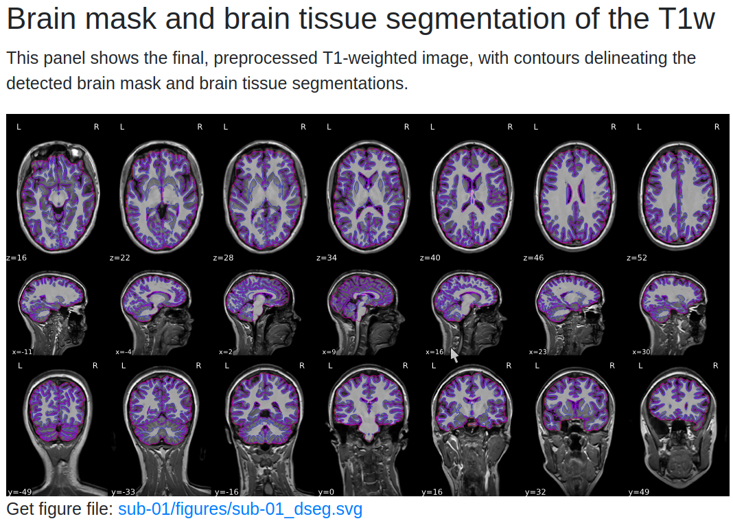
4. Anatomical Quality Checks
The Anatomical section provides:
- Brain Mask Overlay: Displays the brain mask (red outline), gray matter (magenta), and white matter boundaries (blue) overlaid on the anatomical image in sagittal, axial, and coronal views.
-
Normalization Check: A GIF compares the subject’s anatomical image with the MNI template. Ensure that:
-
The outlines of the brain and internal structures (e.g., ventricles) align well.
- Any misalignment could indicate poor normalization, which may need further inspection.
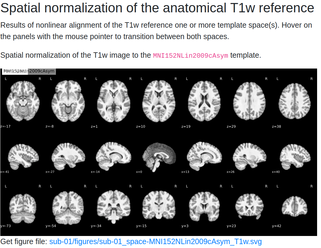
Tip
Hover over the GIF to see the back-and-forth comparison between the subject's brain and the template. Look closely at the alignment of internal brain structures.
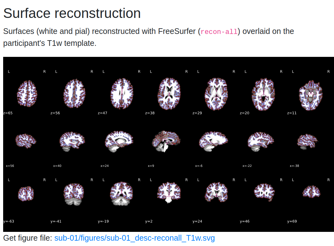
- Surface Reconstruction if you ran the
recon-allroutine in fMRIprep
5. Functional Quality Checks
In the Functional section, you’ll find:
- Functional-to-Anatomical Alignment: A GIF shows how well the preprocessed functional images align with the anatomical image.
Check for alignment
Check for alignment between internal structures like ventricles in the functional and anatomical images. Open the image in a new tab (Right Click on the image -> Open in a new tab) and hover to see the dynamic image.

- CompCor Masks: Displays masks used for Anatomical Component Correction (aCompCor):
- White Matter and CSF (Magenta): Masks used to extract noise components.
- High-Variance Voxels (Blue): Used for Functional Component Correction (fCompCor).
Assessing Alignment
Good alignment between functional and anatomical images is crucial for accurate analysis. Pay special attention to lighter fluid-filled regions in the functional image, which should correspond with dark CSF areas in the anatomical image.
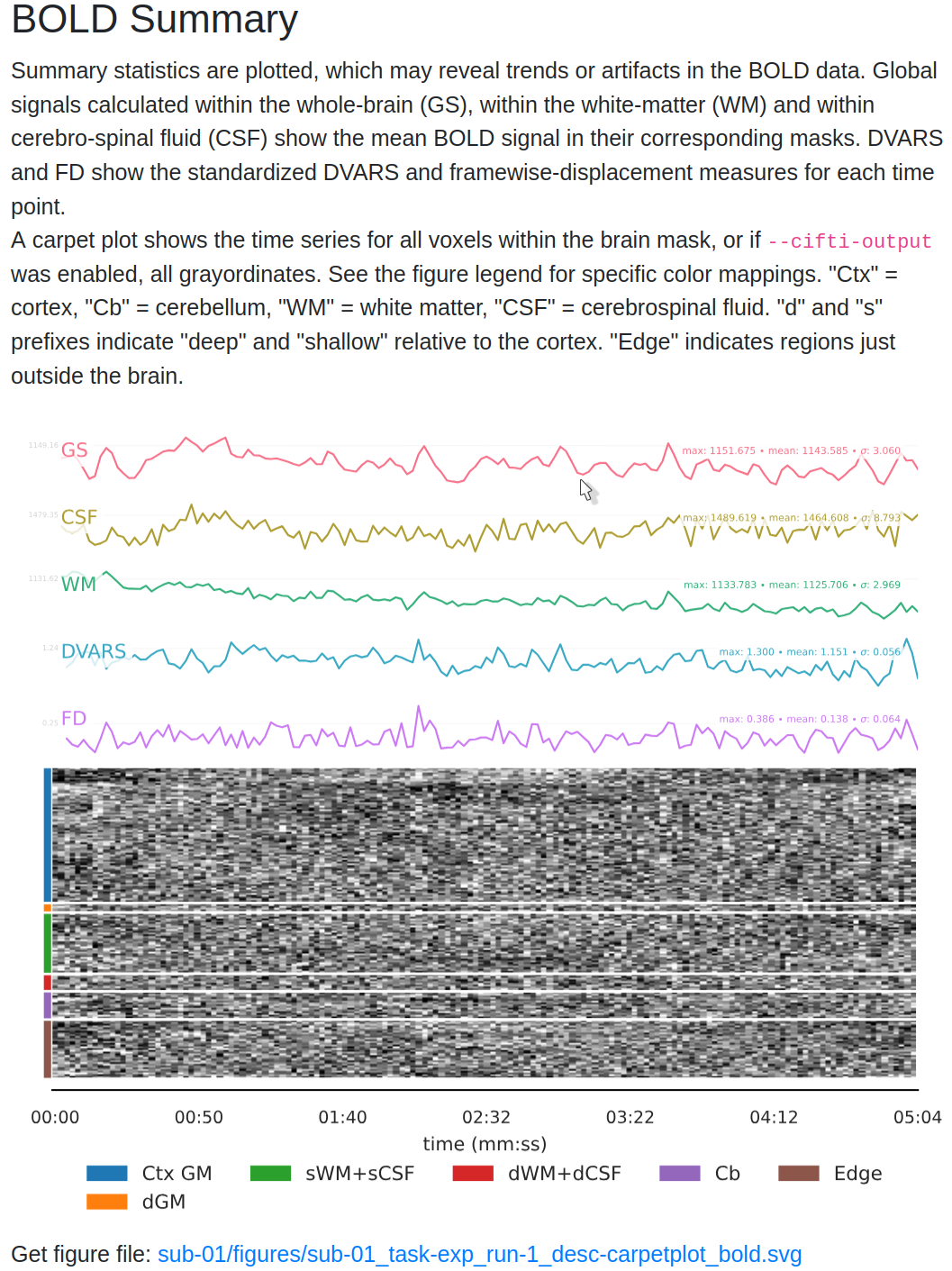
6. BOLD Summary and Carpet plot
The report includes time series plots for various confounds:
- Global Signal (GS): Measures signal fluctuations across the entire brain.
- CSF Signal (GSCSF) and White Matter Signal: Represent fluctuations in specific tissue types.
- Motion Metrics (DVARS, Framewise Displacement):
- DVARS: Shows changes in BOLD signal intensity from one time point to the next.
- Framewise Displacement (FD): Tracks the amount of head movement between frames.
- Use DVARS and FD to identify frames with high motion that could affect data quality.
Tip
High motion values often correlate with changes in global signal. Consider including these regressors in your GLM to account for motion-related noise.
The carpet plot displays time series of BOLD signals across different brain regions:
- Cortex (blue), Subcortex (orange), Gray Matter (green), and White Matter/CSF (red).
- Look for sudden changes across a column, which may indicate motion artifacts affecting the entire brain at a particular time point.
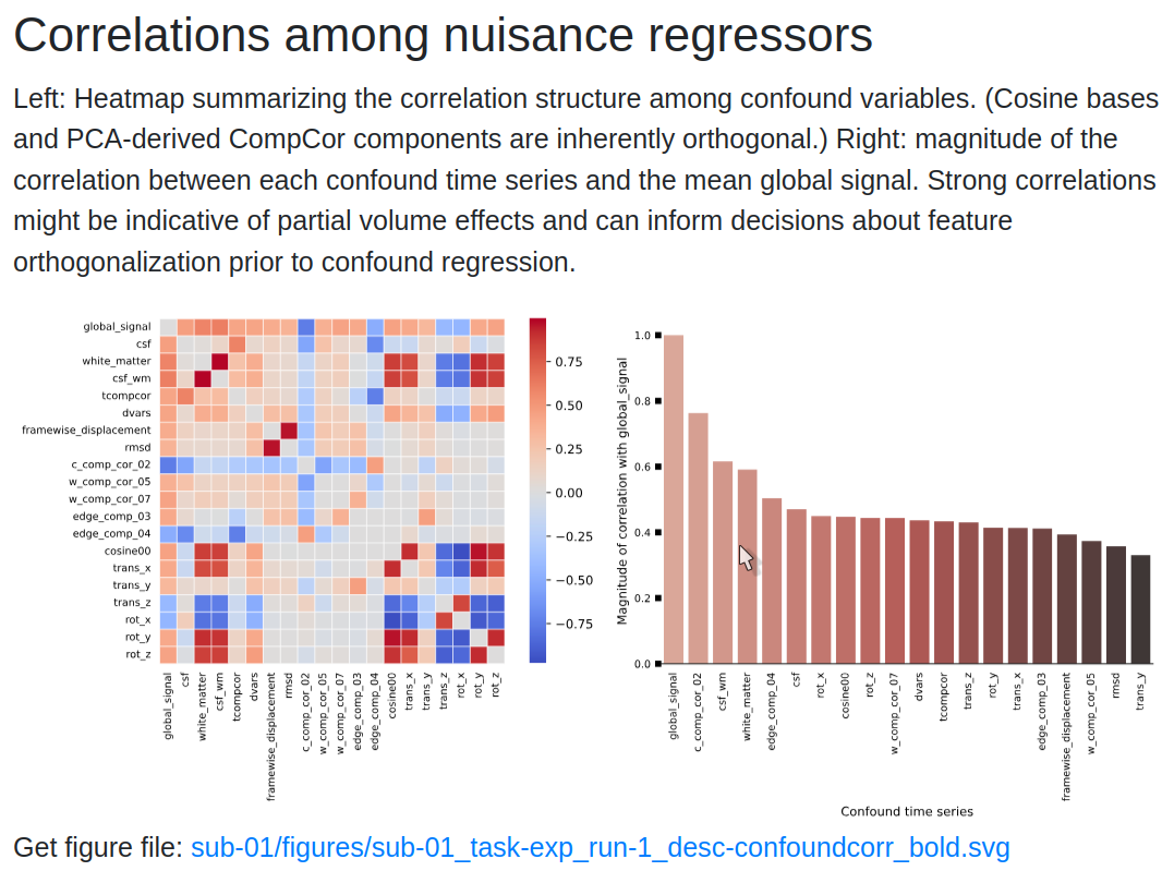
7. Correlation Matrix of Confound Regressors
The report also includes a correlation matrix showing relationships between confound regressors:
- High correlations between CSF and motion regressors may indicate that motion affects CSF signals.
- Use this matrix to decide which regressors to include in your GLM for better noise correction.
High Correlations
High correlation values may suggest redundancy among some regressors. Consider removing or combining them to avoid overfitting when building your GLM.
8. Making Decisions for Further Analysis
After reviewing the report:
- Identify Good Quality Runs: Look for well-aligned images and minimal motion artifacts.
- Decide on Regressors: Choose confounds like DVARS, FD, and CompCor components to include in your GLM.
What confound regressors should I use in my GLM?
A common choice is to include at least the 6 Head Motion parameters, and optionally FD and Global Signal ad nuisance regressors in your GLM.
See this awesome NeuroStars conversation with advice on choosing regressors and relevant resources.
For more details on interpreting fMRIPrep reports, see the fMRIPrep Outputs Documentation and discussions on NeuroStars.
MRIQC HTML Report
The MRIQC report highlights:
- Summary Image: A visual overview of key metrics, including signal-to-noise ratio (SNR) and temporal SNR (tSNR).
- Detailed Metrics: Click through different tabs to examine metrics like Mean Framewise Displacement, EPI-to-T1w registration quality, and artifact presence.
Interpreting tSNR
Higher temporal SNR (tSNR) values indicate better data quality. Typical values range from 30-60 for fMRI. Low tSNR may suggest issues like excessive noise or scanner artifacts. Review the group-level metrics to identify subjects with unusually high motion or low tSNR.
For more information on understanding these metrics, check out the MRIQC interpretation guide on NeuroStars.
Common Issues with fMRIPrep and MRIQC
Memory Errors: Out of Memory (OOM) or Crash
- Problem: fMRIPrep crashes or terminates unexpectedly due to insufficient memory.
- Solution: Reduce the
--mem-mbparameter to allocate less memory or increase the swap space available on your system. This can help prevent OOM errors. - Tip: Monitor your memory usage during processing using tools like
htop(Linux) or Activity Monitor (Mac). Aim to use around 80-90% of your available RAM without exceeding it.
Docker File Permissions Error
- Problem: fMRIPrep cannot access input or output directories due to file permissions.
- Solution: Ensure that Docker has read and write permissions to the directories being mounted. Adjust permissions using:
- Tip: On Windows, ensure that Shared Drives are enabled in Docker Desktop settings.
Missing Fields in JSON Files
- Problem: fMRIPrep fails due to missing
SliceTimingorPhaseEncodingDirectionfields in the JSON sidecar files. - Solution: Verify that all required metadata fields are present using the BIDS Validator. For guidance on JSON sidecar fields, see the BIDS Specification.
- Tip: If using custom acquisition parameters, manually edit JSON files to include the missing fields.
RuntimeError: Fieldmap Issues
- Problem: fMRIPrep throws a
RuntimeErrorrelated to fieldmaps, such as missing or improperly specified fieldmaps. - Solution: Ensure that fieldmaps are correctly specified in your BIDS dataset according to the BIDS Fieldmap documentation.
- Tip: If your study does not require fieldmap correction, you can skip this step by specifying
--ignore fieldmapsin your fMRIPrep command.
MRIQC: NaN Values in JSON Files
- Problem: MRIQC fails when encountering
NaNvalues in JSON metadata files. - Solution: Use a script like
sanitize_json.pyto replaceNaNvalues with valid placeholders before running MRIQC. - Tip: Validate your JSON files before running MRIQC to avoid processing interruptions.
Docker: Cannot Allocate Memory
- Problem: fMRIPrep crashes with the error
cannot allocate memorywhen using Docker. - Solution: Restart the Docker service or allocate more memory and CPUs through the Docker Desktop settings under Resources.
- Tip: Increase memory allocation gradually (e.g., 2-4 GB increments) until fMRIPrep runs smoothly.
Slow Processing: fMRIPrep Takes Too Long
- Problem: fMRIPrep runs slowly, taking an excessively long time for each subject.
- Solution: Use a faster SSD for the
--work-dirto improve read/write speeds and reduce processing time. Also, ensure--n-cpusis set to the majority of available cores, but not all, to avoid system slowdowns. - Tip: Consider running fMRIPrep on a high-performance computing (HPC) cluster if available.
Missing or Corrupted Output Files
- Problem: After running fMRIPrep or MRIQC, certain output files (e.g.,
sub-xx.htmlreports) are missing or corrupted. - Solution: Check for errors in the log files generated during the run. Often, disk space issues or interruptions during processing can cause missing files. Re-run the affected subjects with sufficient disk space.
- Tip: Use a dedicated work directory and ensure it has at least 100 GB of free space to accommodate intermediate files.
MRIQC: No Group Report Generated
- Problem: Group-level analysis in MRIQC does not produce a report.
- Solution: Ensure that MRIQC was run in group mode using the correct
groupargument. Check if all individual reports are present in the output directory before running the group-level command. - Tip: Verify that the
derivatives/mriqcdirectory has read and write access for Docker.
fMRIPrep output: empty surf files
-
Problem: Some files in
freesurfer/sub-xx/surfare empty (0 KB), namely:*h.fsaverage.sphere.reg*h.pial*h.white.H*h.white.K
These files are supposed to be symbolic links pointing to other outputs in the folder. A 0 KB size indicates that the link is broken. This often happens if preprocessing was done on Windows, since Windows does not fully preserve these link-type files.
Even if the symbolic link is broken, the files to which the links originally pointed are likely still present in your
surf/folder, so you do not need to re-runrecon-allorfmriprep. -
Solution: If you need any of these files, you can either use the corresponding “original” file directly, or recreate the symbolic link (or a duplicate file) so external tools can see it under the expected filename. Below are the relevant file mappings:
Broken (link) file Original (target) file *h.fsaverage.sphere.reg*h.sphere.reg*h.pial*h.pial.T1*h.white.K*h.white.preaparc.K*h.white.H*h.white.preaparc.HFor instance, if you need
lh.pialand it’s empty, you can create it by copyinglh.pial.T1with the following command:To fix these links automatically across multiple subjects (on Windows, use the WSL terminal, not in the native PowerShell / Windows terminal)):
- Set your
FREESURFER_PATH(the folder containing your pre-existingrecon-allor output): - Copy and paste the script below into an empty file and save it as
fix_surf_files.sh. - Open a terminal and navigate to the folder where you saved the file (e.g.,
cd ~/Documents). - Make the script executable:
chmod +x fix_surf_files.sh - Run the script:
./fix_surf_files.sh
Here is the full script:
- Set your
With these quality checks complete, you're ready to proceed to the General Linear Model (GLM) analysis. See the next guide for instructions on setting up your GLM. → Go to GLM