fMRI workflow example
This page walks through a complete fMRI analysis pipeline as implemented in a real study on chess expertise. It shows how the individual steps documented throughout this wiki come together in practice — from collecting scans at the hospital all the way to whole-brain decoding results plotted on inflated cortical surfaces.
The full code is available in the chess-expertise-2025 GitHub repository. For setting up your environment and tools, see Set-up your fMRI environment and Coding practices.
Pipeline overview
1. Collecting raw data at the hospital
The first thing you do after a scanning session is collect the data from the hospital computers: fMRI scans (DICOMs), behavioral log files, and — in this study — eye-tracking recordings. Before anything leaves the hospital, you anonymize all filenames to remove any personal identifiers. The raw files are then organized into a sourcedata/ folder with separate subfolders for each data type (nifti/, bh/, et/).
For the practical details of what happens in the scanning room, see Scanning procedure. For how to organize your raw data, see General information.
2. Converting everything to BIDS
With raw data in hand, the next step is converting it all into a standardized BIDS structure. This involves three conversions:
- fMRI data: Use
dicm2niiin MATLAB to convert DICOMs to NIfTI files and generate JSON sidecars. For the first subject, you create template JSON files; subsequent subjects reuse those templates. - Behavioral data: A custom script (
script02) parses the.matlog files from the task and producesevents.tsvfiles withonset,duration, andtrial_typecolumns. - Eye-tracking data: EDF files from the EyeLink system are converted to ASC format using the EyeLink API, then organized following the (still draft) BEP020 convention.
After conversion, always run the BIDS Validator to catch any issues.
Full guide: BIDS conversion, including the eye-tracking section.
3. Quality control with MRIQC
Before investing hours in preprocessing, you want to check data quality. MRIQC generates per-subject quality reports with metrics like SNR, motion estimates, and artifact indicators. You can then run group-level analysis to compare subjects and use the MRIQC classifier to flag problematic datasets. In this study, several subjects were excluded at this stage due to excessive motion.
Commands and interpretation: Preprocessing & QA — MRIQC.
4. Preprocessing with fMRIPrep
fMRIPrep handles the heavy lifting: motion correction, slice timing correction, spatial normalization, and (optionally) surface reconstruction via FreeSurfer. In this pipeline, we requested three output spaces — MNI152NLin2009cAsym:res-2 for group analyses, anat for subject-space analyses, and fsnative for surface data. Processing takes roughly 4–8 hours per subject depending on hardware.
After each subject completes, check the HTML report carefully — especially the registration overlays and framewise displacement plots.
Setup, resource tips, and report interpretation: Preprocessing & QA — fMRIPrep.
5. Eye-tracking extraction with bidsmreye
This study also used bidsmreye, a tool that extracts gaze position directly from the eye region in BOLD images using a deep learning model. It runs as a post-processing step on fMRIPrep outputs and provides eye-tracking estimates even when no external eye-tracker was used (or as a complement to external recordings).
Docker command and usage notes: Preprocessing & QA — bidsmreye.
6. First-level GLM
With preprocessed data, the next step is fitting a General Linear Model (GLM) in SPM to obtain beta images for each experimental condition. A custom script (script03) automates the full pipeline: gunzipping fMRIPrep outputs, optional smoothing, design matrix construction (incorporating confound regressors from fMRIPrep), model estimation, and contrast specification.
After running the GLM, it's important to open SPM's Results interface and verify that the design matrix looks correct: no overlapping conditions, right number of runs, confounds at the end of each run, and contrast weights assigned properly.
Full guide: GLM analysis. For visualizing results on brain volumes or surfaces, see the activation visualization section.
7. Defining ROIs with the Glasser parcellation
For the MVPA, we needed Regions of Interest covering the entire cortex. We used the Glasser2016 parcellation (HCP-MMP1.0), which provides 180 anatomically defined parcels per hemisphere. For this study, we projected the atlas from fsaverage onto each subject's native space using an automated shell script (HPC-to-subject.sh), since we ran analyses in subject space. If you're working in MNI space instead (which is the more common case), a ready-made volumetric MNI atlas is available — see the ROIs page for details.
All ROI methods: ROIs, including the Glasser parcellation section.
8. Whole-brain MVPA decoding
With beta images and ROIs in hand, we ran independent cross-validated SVM classification in each of the 180 Glasser parcels per hemisphere (script04). This tells us which brain regions carry information about the experimental conditions (in this case, chess expertise).
The results are saved as decoding accuracy per ROI in a BIDS-compatible derivatives/mvpa structure.
MVPA concepts and tutorial: MVPA.
9. Hierarchical aggregation, significance testing, and visualization
The Glasser parcellation has a built-in hierarchy: the 180 fine-grained parcels group into larger cortical regions, which in turn group into broad cortical divisions. We leveraged this by running the analysis at the finest level and then aggregating upward (script06):
- Fine-grained (Level 1): Decoding accuracy in each of the 180 parcels per hemisphere.
- Intermediate (Level 2): Averaged accuracy across parcels belonging to the same larger region.
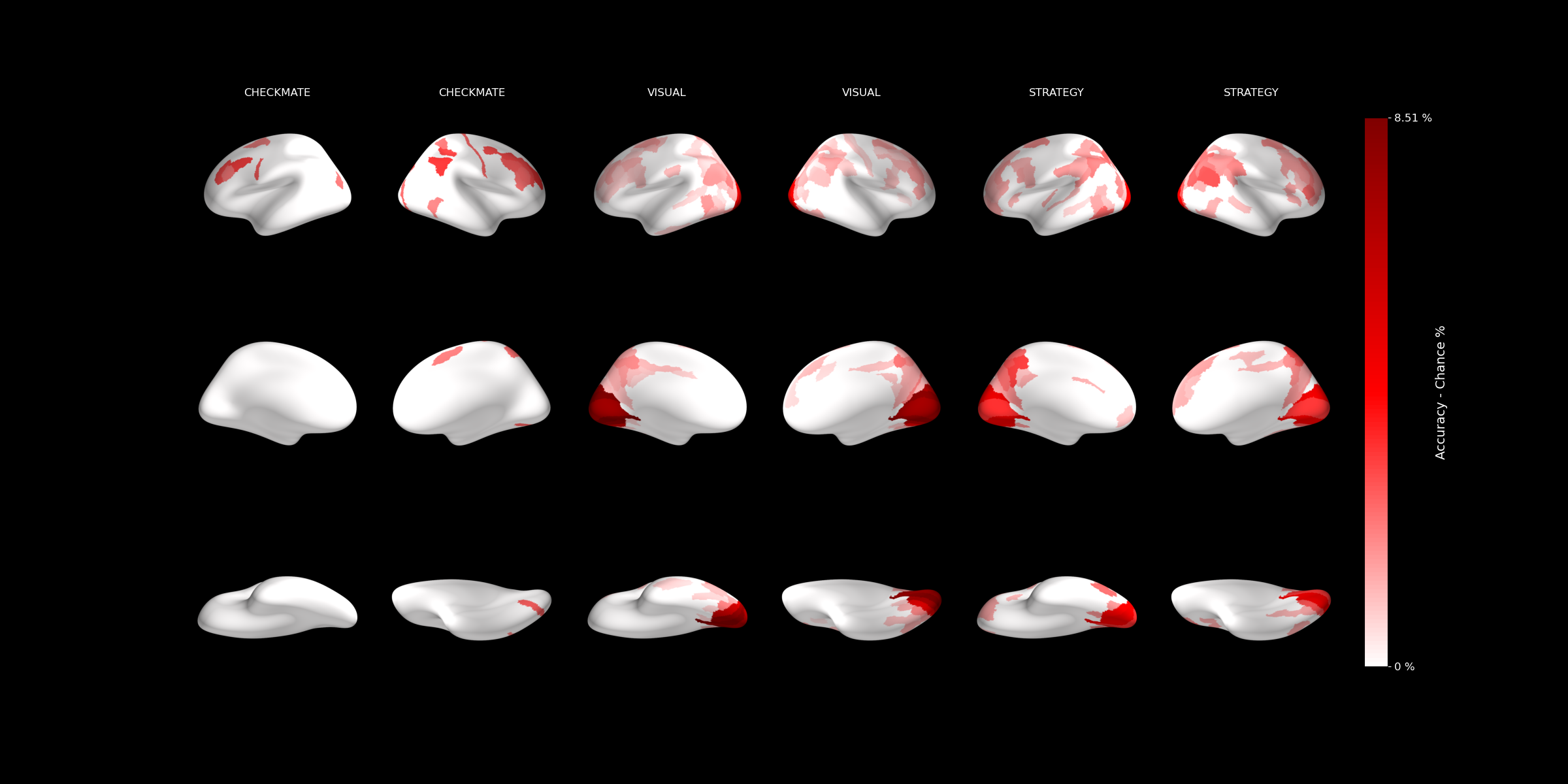
- Coarse (Level 3): Averaged across broad cortical divisions.
At each level, significance was tested against chance, and the results were plotted on inflated brain surfaces: